Soft Drink Delivery Times

Keywords: linear regression, influence, outliers, gamma regression.

Description

A soft drink bottler is analyzing vending machine service routes in his distribution system. He is interested in predicting the amount of time required by the route driver to service the vending machines in an outlet. This service activity including stocking the machine with beverage products and minor maintenance or housekeeping. The industrial engineer responsible for the study has suggested that the two most important variables affecting the delivery time are the number of cases of product stocked and the distance walked by the route driver. The engineer has collected 25 observations on delivery time (minutes), number of cases and distance walked (feet).

Download

Data File (tab-delimited text)

Source

Montgomery, D. C., and Peck, E. A. (1992). Introduction to Regression Analysis. Wiley, New York. Example 4.1

Analysis

The data is highly skew without transformation. Montgomery and Peck use it to illustrate influence and outlier measures.

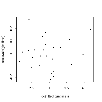
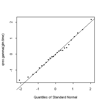
A gamma regression model fits well. One might expect the intercept to be zero, but this does not appear to be the case. There is no evidence of any dispersion effects.

> glm.time <- glm(Time~Cases+Distance,family=tweedie(var.power=2,link.power=1))
> summary(glm.time)

Call: glm(formula = Time ~ Cases + Distance, family = tweedie(var.power = 2,
	link.power = 1))
Deviance Residuals:
        Min          1Q      Median         3Q       Max
 -0.2172532 -0.09177765 -0.01094719 0.04847197 0.2778221

Coefficients:
                 Value Std. Error  t value
(Intercept) 4.39767525 0.78103500 5.630574
      Cases 1.55172654 0.16941397 9.159378
   Distance 0.01006716 0.00285558 3.525434

(Dispersion Parameter for Tweedie family taken to be 0.017002 )

    Null Deviance: 7.705974 on 24 degrees of freedom

Residual Deviance: 0.3661046 on 22 degrees of freedom

Number of Fisher Scoring Iterations: 3

Correlation of Coefficients:
         (Intercept)      Cases
   Cases -0.5352342
Distance -0.1580529  -0.6442069
> plot(log(fitted(glm.time)),residuals(glm.time))

> qqnorm(qres.gamma(glm.time))

> abline(0,1)
> dglm.time <- dglm(Time~Cases+Distance,~Cases+Distance,method="ml",family=tweedie(var.power=2,link.power=1))
> anova(dglm.time)
Analysis of Deviance Table

Tweedie double generalized linear model

Response: Time

                 DF Seq.Chisq         P Adj.Chisq         P
      Mean model  2  76.17080 0.0000000  62.36841 0.0000000
Dispersion model  2   0.32317 0.8507928   0.32317 0.8507928